4. Basic Usage
4.1. A First Calculation
We’re now ready to start using NumBAT.
Let’s jump straight in and run a simple calculation. Later in the chapter, we go deeper into some of the details that we will encounter in this first example.
4.1.1. Tutorial 1 – Basic SBS Gain Calculation
Simulations with NumBAT are generally carried out using a python script file.
This example, contained in <NumBAT>examples/tutorials/sim-tut_01-first_calc.py calculates the backward SBS gain for a rectangular silicon waveguide surrounded by air.
Move into the examples/tutorials directory and then run the script by entering:
$ python3 sim-tut_01-first_calc.py
After a short while, you should see some values for the SBS gain printed to the screen. In many more examples/tutorials in the subsequent chapters, we will meet much more convenient forms of output, but for now let’s focus on the steps involved in this basic calculation.
The sequence of operations (annotated in the source code below as Step 1, Step 2, etc) is:
Add the NumBAT install directory to Python’s module search path and then import the NumBAT python modules.
Set parameters to define the structure shape and dimensions.
Set parameters determining the range of electromagnetic and elastic modes to be solved.
Create the primary
NumBATAppobject to access most NumBAT features and set the filename prefix for all outputs.Construct the waveguide with
nbapp.make_structureout of a number ofmaterials.Materialstructure.Generate output files containing images of the finite element mesh and final refractive index. These are illustrated in figures below.
Solve the electromagnetic problem at a given free space wavelength \(\lambda\). The function
modecalcs.calc_EM_modes()returns anEMSimResultobject containing electromagnetic mode profiles, propagation constants, and potentially other data which can be accessed through various methods we will meet in later examples/tutorials. The calculation is provided with a rough estimate of the effective index to guide the solver the find guided eigenmodes in the desired part of the spectrum. After the calculation, we can obtain the exact effective index of the fundamental mode usingmodecalcs.neff().Display the propagation constants in units of \(\text{m}^{-1}\) of the EM modes using
modecalcs.kz_EM_all()Calculate the electromagnetic fields for the Stokes mode. As the pump and Stokes frequencies are very similar, the Stokes modes can be found with high precision by a simple complex conjugate transformation of the pump fields.
Identify the desired elastic wavenumber from the difference of the pump and Stokes propagation constants and solve the elastic problem.
modecalcs.calc_AC_modes()returns anACSimResultobject containing the elastic mode profiles, frequencies and potentially other data at the specified propagation constantk_AC.Display the elastic frequencies in Hz using
modecalcs.nu_AC_all().Use
integration.get_gains_and_qs()to generate aGainPropsobject containing information on the total SBS gain, contributions from photoelasticity and moving boundary effects, and the elastic loss.Extract desired values from the gain properties and print them to the screen.
You may have noticed from this description that the eigenproblems for the electromagnetic and acoustic problems are framed in opposite senses. The electromagnetic problem finds the wavenumbers \(k_{z,n}(\omega)\) (or equivalently the effective indices) of the modes at a given free space wavelength (ie. at a specified frequency \(\omega=2\pi c/\lambda\)). The elastic solver, however, works in the opposite direction, finding the elastic modal frequencies \(\nu_n(q_0)\) at a given elastic propagation constant \(q_0\). While this might seem odd at first, it is actually the natural way to frame SBS calculations.
We emphasise again, that for convenience, the physical dimensions of waveguides are specified in nanometres. All other quantities in NumBAT are expressed in the standard SI base units.
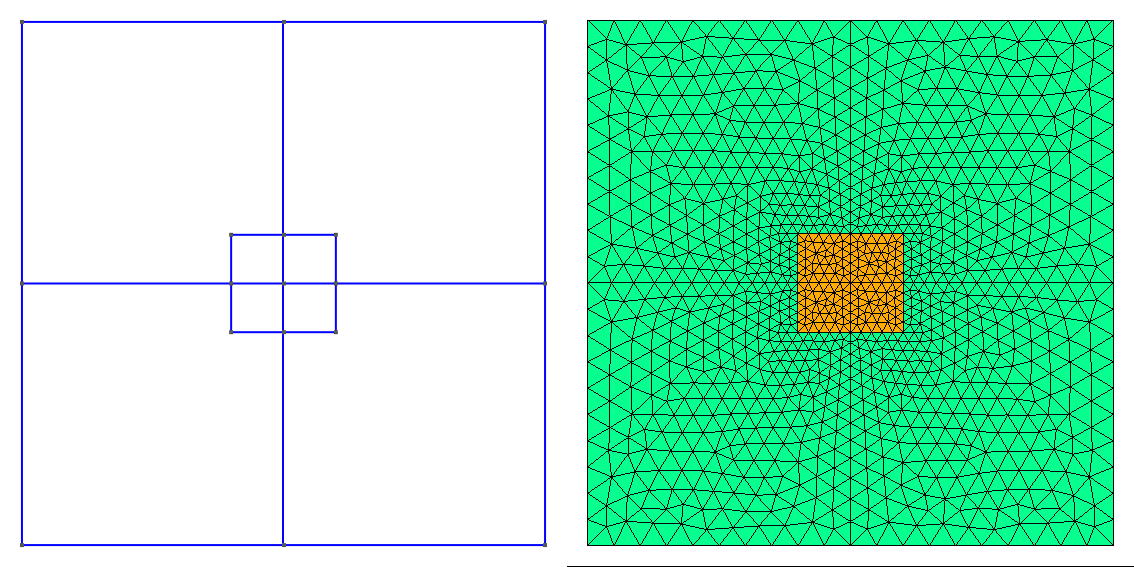
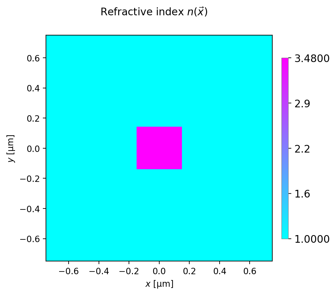
Generated meshes and refractive index profile.
Here’s the full source code for this tutorial:
print(nbapp.final_report())
""" Calculate the backward SBS gain for modes in a
    silicon waveguide surrounded in air.
"""

# Step 1
import sys
import numpy as np

from pathlib import Path
sys.path.append(str(Path('../../backend')))


import numbat
import integration

import materials


# Naming conventions
# AC: acoustic
# EM: electromagnetic
# q_AC: acoustic wavevector

print('\n\nCommencing NumBAT tutorial 1')

# Step 2
# Geometric Parameters - all in nm.

lambda_nm = 1550.0  # Wavelength of EM wave in vacuum.

# Waveguide widths.
inc_a_x = 300.0
inc_a_y = 280.0

# Unit cell must be large to ensure fields are zero at boundary.
domain_x = 1500.0
domain_y = domain_x


# Shape of the waveguide.
inc_shape = 'rectangular'

# Step 3
# Number of electromagnetic modes to solve for.
num_modes_EM_pump = 20
num_modes_EM_Stokes = num_modes_EM_pump

# Number of acoustic modes to solve for
num_modes_AC = 20

# The EM pump mode(s) for which to calculate interaction with AC modes.
# Can specify a mode number (zero has lowest propagation constant) or 'All'.
EM_mode_index_pump = 0
# The EM Stokes mode(s) for which to calculate interaction with AC modes.
EM_mode_index_Stokes = 0
# The AC mode(s) for which to calculate interaction with EM modes.
AC_mode_index = 'All'

# Step 4
# Create the primary NumBAT application object and set the file output prefix
prefix = 'tut_01'
nbapp = numbat.NumBATApp(prefix)

# Step 5
# Use specified parameters to create a waveguide object.
# to save the geometry and mesh as png files in backend/fortran/msh/

wguide = nbapp.make_structure(inc_shape, domain_x, domain_y, inc_a_x, inc_a_y,
                           material_bkg=materials.make_material("Vacuum"),
                           material_a=materials.make_material("Si_2016_Smith"),
                           lc_bkg=.05,  # in vacuum background
                           lc_refine_1=2.5,  # on cylinder surfaces
                           lc_refine_2=2.5)  # on cylinder center

# Step 6
# Optionally output plots of the mesh and refractive index distribution
wguide.plot_mesh(prefix)
wguide.plot_refractive_index_profile(prefix)

# Step 7
# Calculate the Electromagnetic modes of the pump field.

# We provide an estimated effective index of the fundamental guided mode to steer the solver.
n_eff = wguide.get_material('a').refindex_n-0.1

sim_EM_pump = wguide.calc_EM_modes(num_modes_EM_pump, lambda_nm, n_eff)

# Report the exact effective index of the fundamental mode
n_eff_sim = np.real(sim_EM_pump.neff(0))
print("\n Fundamental optical mode ")
print(" n_eff = ", np.round(n_eff_sim, 4))


# Step 8
# Display the wavevectors of EM modes.
v_kz = sim_EM_pump.kz_EM_all()
print('\n k_z of electromagnetic modes [1/m]:')
for (i, kz) in enumerate(v_kz):
    print(f'{i:3d}  {np.real(kz):.4e}')

# Step 9
# Calculate the Electromagnetic modes of the Stokes field.
# For an idealised backward SBS simulation the Stokes modes are identical
# to the pump modes but travel in the opposite direction.
sim_EM_Stokes = sim_EM_pump.clone_as_backward_modes()

# Alternatively, solve again directly
# sim_EM_Stokes = wguide.calc_EM_modes(lambda_nm, num_modes_EM_Stokes, n_eff, Stokes=True)


# Step 10
# Calculate Acoustic modes, using the mesh from the EM calculation.

# Find the required acoustic wavevector for backward SBS phase-matching
q_AC = np.real(sim_EM_pump.kz_EM(0) - sim_EM_Stokes.kz_EM(0))

print('\n Acoustic wavenumber (1/m) = ', np.round(q_AC, 4))

sim_AC = wguide.calc_AC_modes(num_modes_AC, q_AC, EM_sim=sim_EM_pump)

# Step 11
# Print the frequencies of AC modes.
v_nu = sim_AC.nu_AC_all()
print('\n Freq of AC modes (GHz):')
for (i, nu) in enumerate(v_nu):
    print(f'{i:3d}  {np.real(nu)*1e-9:.5f}')


# Step 12

# Do not calculate the acoustic loss from our fields, instead set a Q factor.
set_q_factor = 1000.

# Calculate interaction integrals and SBS gain for PE and MB effects combined,
# as well as just for PE, and just for MB. Also calculate acoustic loss alpha.


gain = integration.get_gains_and_qs(
    sim_EM_pump, sim_EM_Stokes, sim_AC, q_AC, EM_mode_index_pump=EM_mode_index_pump,
    EM_mode_index_Stokes=EM_mode_index_Stokes, AC_mode_index=AC_mode_index, fixed_Q=set_q_factor)

# Step 13
# SBS_gain_tot, SBS_gain_PE, SBS_gain_MB are 3D arrays indexed by pump, Stokes and acoustic mode
# Extract those of interest as a 1D array:

SBS_gain_PE_ij = gain.gain_PE_all_by_em_modes(EM_mode_index_pump, EM_mode_index_Stokes)
SBS_gain_MB_ij = gain.gain_MB_all_by_em_modes(EM_mode_index_pump, EM_mode_index_Stokes)
SBS_gain_tot_ij = gain.gain_total_all_by_em_modes(EM_mode_index_pump, EM_mode_index_Stokes)

# Print the Backward SBS gain of the AC modes.
print("\nContributions to SBS gain [1/(WM)]")
print("Acoustic Mode number | Photoelastic (PE) | Moving boundary(MB) | Total")

for (m, gpe, gmb, gt) in zip(range(num_modes_AC), SBS_gain_PE_ij, SBS_gain_MB_ij, SBS_gain_tot_ij):
    print(f'{m:8d}  {gpe:18.6e}  {gmb:18.6e}  {gt:18.6e}')


# Mask negligible gain values to improve clarity of print out.
threshold = 1e-3
masked_PE = np.where(np.abs(SBS_gain_PE_ij) > threshold, SBS_gain_PE_ij, 0)
masked_MB = np.where(np.abs(SBS_gain_MB_ij) > threshold, SBS_gain_MB_ij, 0)
masked_tot = np.where(np.abs(SBS_gain_tot_ij) > threshold, SBS_gain_tot_ij, 0)

print("\n Displaying gain results with negligible components masked out:")

print("AC mode | Photoelastic (PE) | Moving boundary(MB) | Total")
for (m, gpe, gmb, gt) in zip(range(num_modes_AC), masked_PE, masked_MB, masked_tot):
    print(f'{m:8d}  {gpe:12.4f}  {gmb:12.4f}  {gt:12.4f}')

print(nbapp.final_report())
In the next few chapters, we meet many more examples that show the different capabilities of NumBAT and provided comparisons against analytic and experimental results from the literature.
For the remainder of this chapter, we will explore some of the details involved in specifying a wide range of waveguide structures.
4.2. General Simulation Procedures
Simulations with NumBAT are generally carried out using a python script file. This file is kept in its own directory which may or may not be within your NumBAT tree. All results of the simulation are automatically created within this directory. This directory then serves as a complete record of the calculation. Often, we will also save the simulation structure within this directory for future inspection, manipulation, plotting, etc.
These files can be edited using your choice of text editor (for instance nano or vim) or an IDE (for instance MS Visual Code or pycharm) which allow you to run and debug code within the IDE.
To save the results from a simulation that are displayed upon execution (the print statements in your script) use:
$ python3 ./sim-tut_01-first_calc.py | tee log-simo.log
To have direct access to the simulation structure upon the completion of a script use:
$ python3 -i ./sim-tut_01-first_calc.py
This will execute the python script and then return you into an interactive python session within the terminal. This terminal session provides the user experience of an ipython type shell where the python environment and all the simulation structure are in the same state as in the script when it has finished executing. In this session you can access the docstrings of structure, classes and methods. For example:
>>> from pydoc import help
>>> help(structure.Structure)
where we have accessed the docstring of the Struct class from structure.py.
4.3. Script Structure
As with our first example above, most NumBAT scripts proceed with a standard structure:
importing NumBAT modules
defining materials
defining waveguide geometries and associating them with material properties
solving electromagnetic and acoustic modes
calculating gain and other derived quantities