6. Materials, waveguides and meshing

Now that we have a basic understanding of using NumBAT, this chapter provides detailed information on how to specify a large of range materials and waveguide designs.

We will return to more advanced examples/tutorials in the next chapter.

6.1. Materials

In order to calculate the modes of a structure we must specify the acoustic and optical properties of all constituent materials.

In NumBAT, this data is read in from human-readable .json files, which are stored in the directory <NumBAT>/backend/material_data.

These files not only provide the numerical values for optical and acoustic variables, but provide links to the origin of the data. Often they are taken from the literature and the naming convention allows users to select from different parameter values chosen by different authors for the same nominal material.

The intention of this arrangement is to create a library of materials that can serves as standard reference data within the research community. They also allow users to check the sensitivity of their results on particular parameters for a given material.

At present, the library contains the following materials:

• Vacuum (or air)

  • Vacuum

• The chalcogenide glass Arsenic tri*sulfide

  • As2S3_2016_Smith

  • As2S3_2017_Morrison

  • As2S3_2021_Poulton

• Fused silica

  • SiO2_2013_Laude

  • SiO2_2015_Van_Laer

  • SiO2_2016_Smith

  • SiO2_2021_Smith

  • SiO2_smf28.json

  • SiO2GeO2_smf28.json

• Silicon

  • Si_2012_Rakich

  • Si_2013_Laude

  • Si_2015_Van_Laer

  • Si_2016_Smith

  • Si_2021_Poulton

  • Si_test_anisotropic

• Silicon nitride

  • Si3N4_2014_Wolff

  • Si3N4_2021_Steel

• Gallium arsenide

  • GaAs_2016_Smith

• Germanium

  • Ge_cubic_2014_Wolff

• Lithium niobate

  • LiNbO3_2021_Steel

  • LiNbO3aniso_2021_Steel

Materials can easily be added to this library by copying any of these files as a template and modifying the properties to suit. The Si_test_anisotropic file contains all the variables that NumBAT is setup to read. We ask that stable parameters (particularly those used for published results) be added to the NumBAT git repository using the same naming convention.

6.2. Waveguide Geometries

NumBAT encodes different waveguide structures through finite element meshes constructed using the .geo language used by the open source tool Gmsh. Most users will find they can construct all waveguides of interest using the existing templates. However, new templates can be added by adding a new .geo file to the <NumBAT>/backend/fortran/msh directory and making a new subclass of the UserGeometryBase class in the <NumBAT>/backend/msh/user_meshes.py file. This procedure is described in detail in User-defined waveguide geometries.

All the builtin examples below are constructed in the same fashion in a parallel builtin_meshes.py file and can be used as models for your own designs.

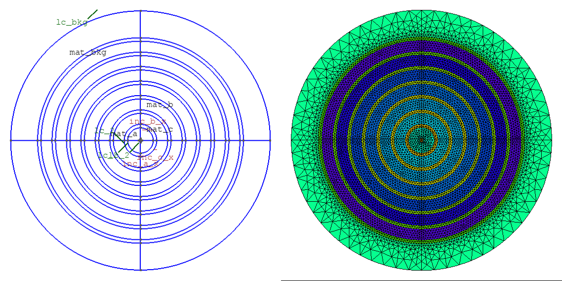
The following figures give some examples of how material types and physical dimensions are represented in the mesh geometries. In particular, for each structure template, they identify the interpretation of the dimensional parameters (inc_a_x, slab_b_y, etc), material labels (material_a, material_b etc), and the grid refinement parameters (lc_bkg, lc_refine_1, lc_refine_2, etc). The captions for each structure also identify the mesh geometry template files in the directory <NumBAT>/backend/fortran/msh with filenames of the form <prefix>_msh_template.geo which define the structures and can give ideas for developing new structure files.

The NumBAT code for creating all these structures can be found in <NumBAT>/docs/source/images/make_meshfigs.py.

6.2.1. Single inclusion waveguides with surrounding medium

These structures consist of a single medium inclusion (mat_a) with a background material (mat_bkg). The dimensions are set with inc_a_x and inc_a_y.

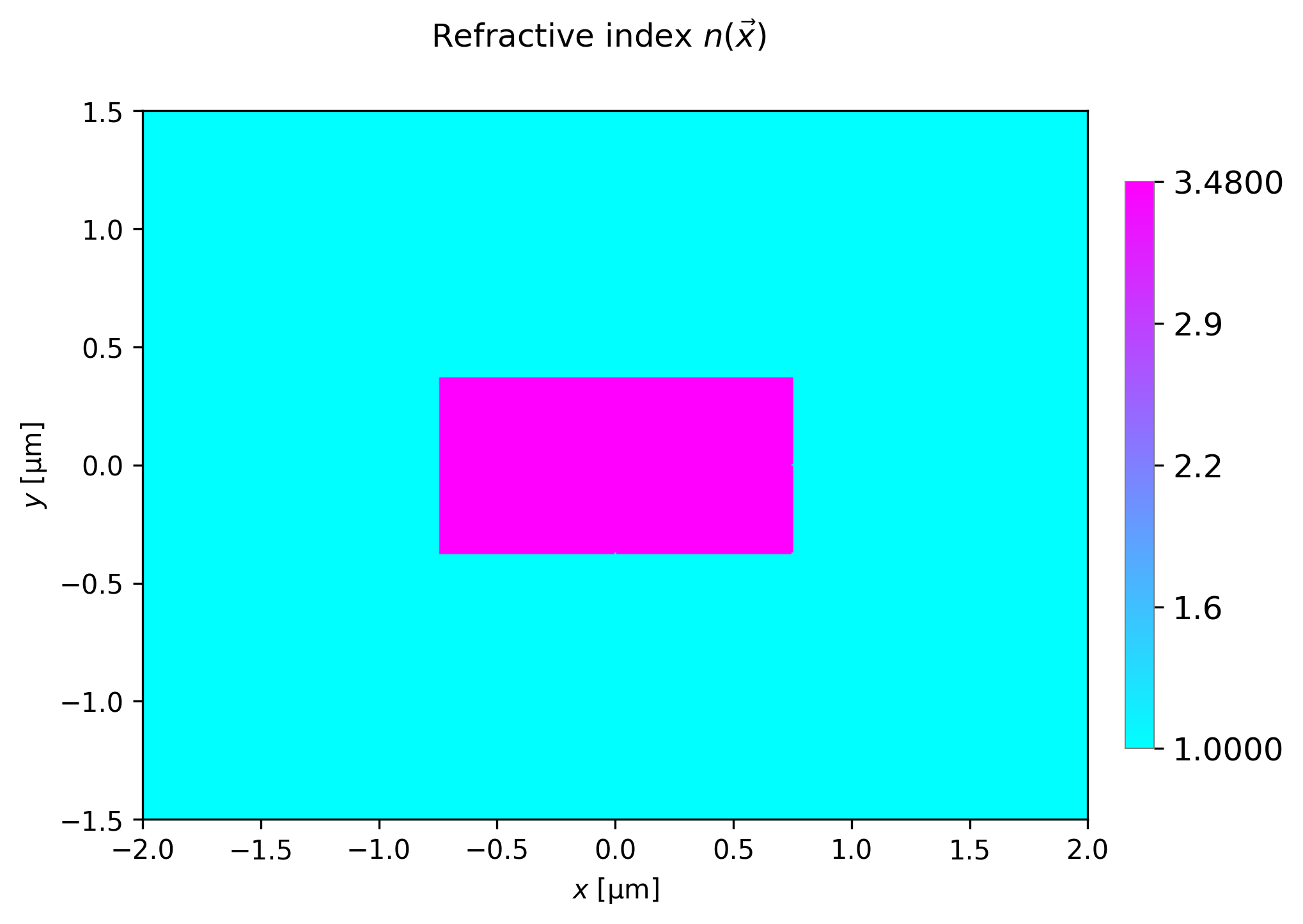
Rectangular waveguide using shape rectangular (template oneincl_msh).

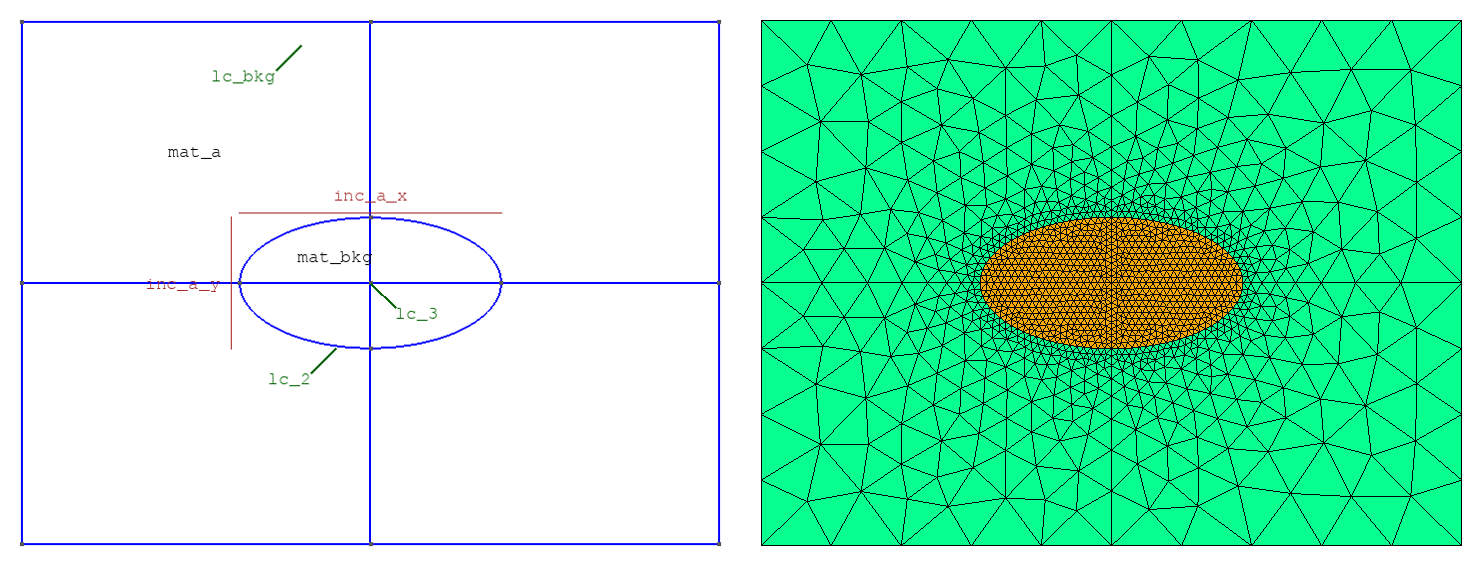
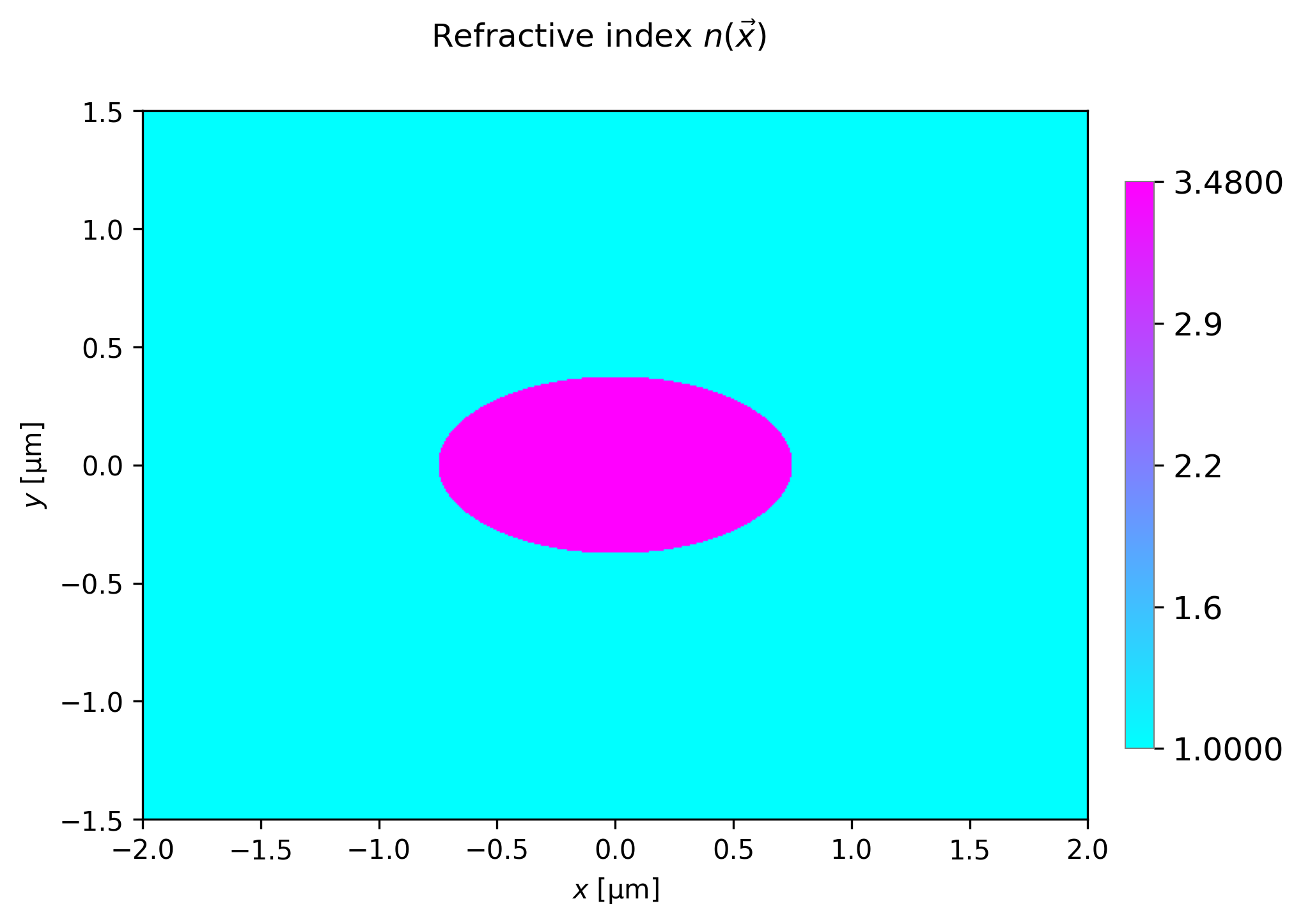
Elliptical waveguide using shape circular (template oneincl_msh).

Triangular waveguide using shape triangular.

6.2.2. Double inclusion waveguides with surrounding medium

These structures consist of a pair of waveguides with a single common background material. The dimensions are set by inc_a_x/inc_a_y and inc_b_x/inc_b_y. They are separated horizontally by two_inc_sep and the right waveguide has a vertical offset of y_off.

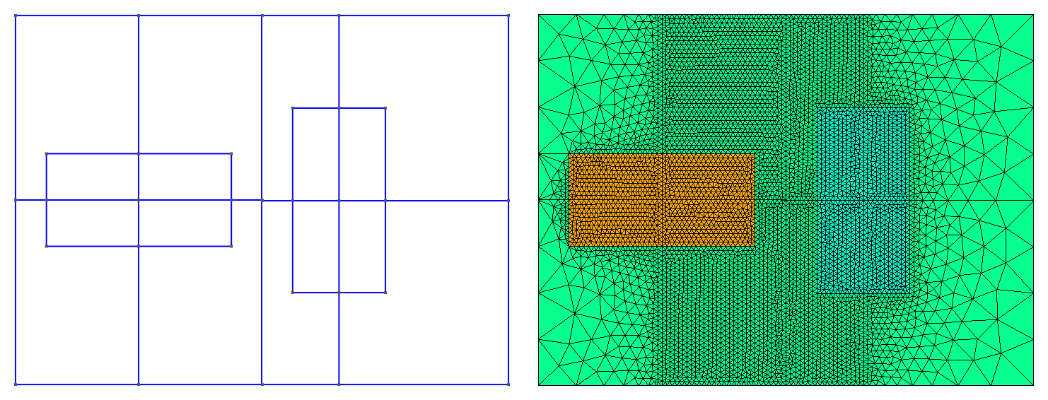
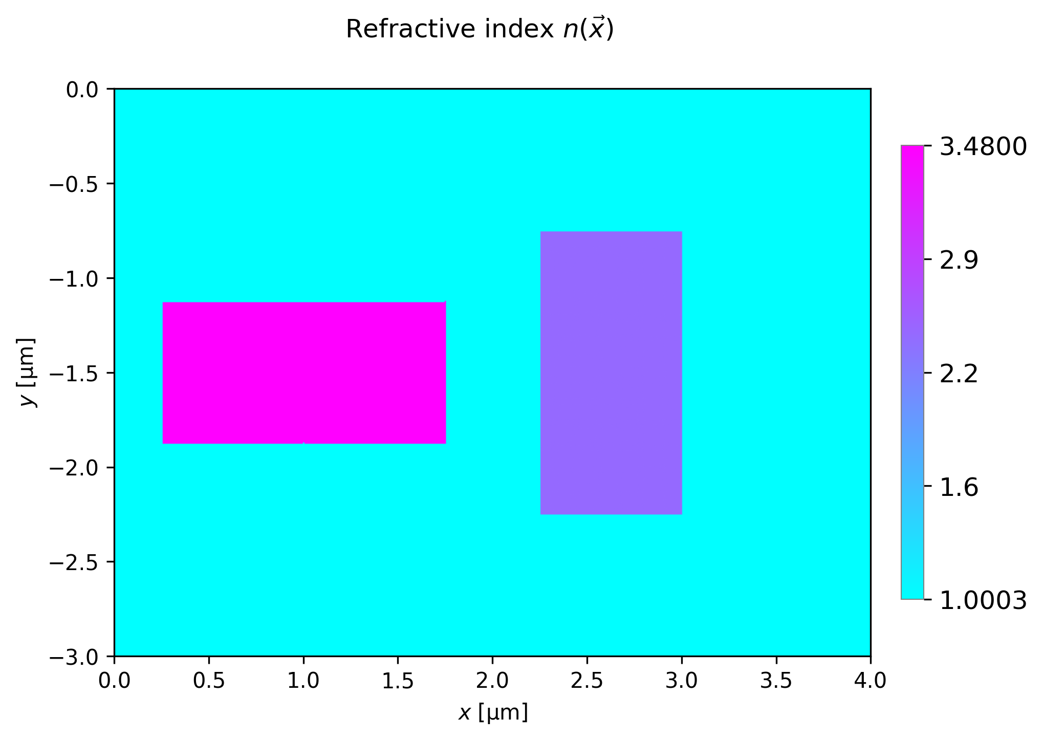
Coupled rectangular waveguides using shape rectangular (template twoincl_msh).

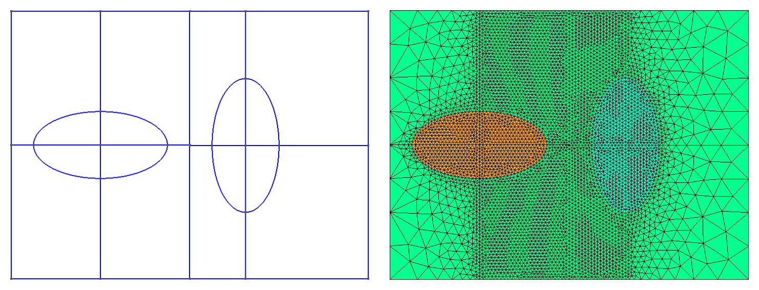
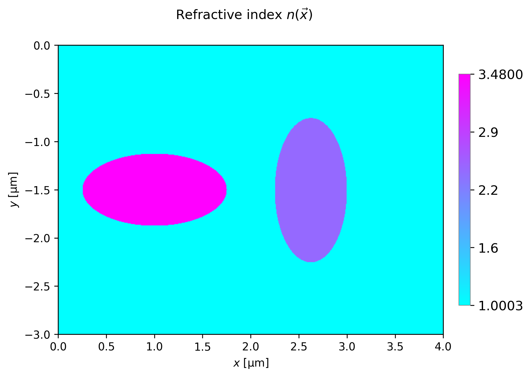
Coupled circular waveguides using shape circular (template twoincl_msh). There appears to be a bug here!

6.2.3. Rib waveguides

These structures consist of a rib on one or more substrate layers with zero to two coating layers.

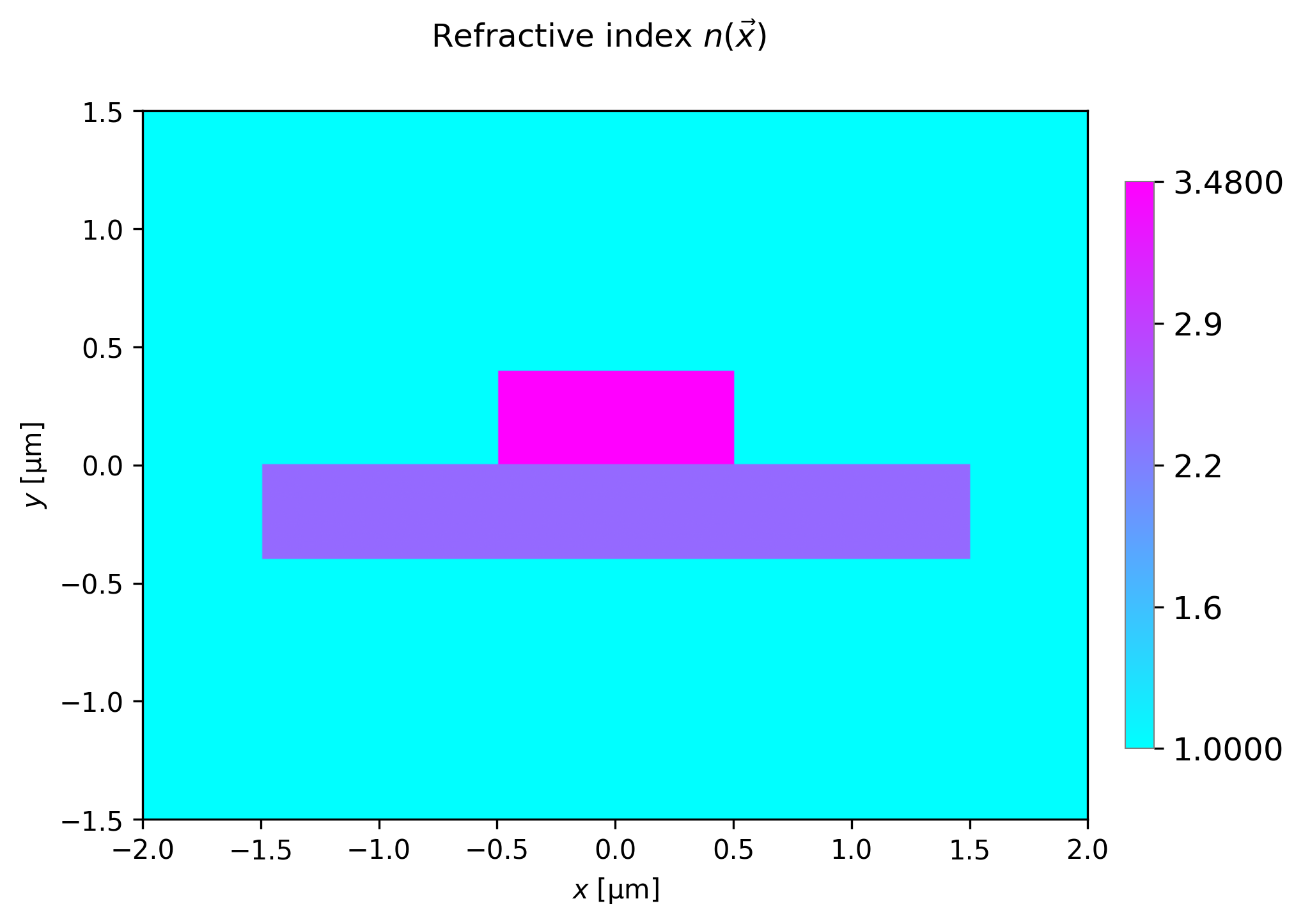
A conventional rib waveguide using shape rib (template rib).

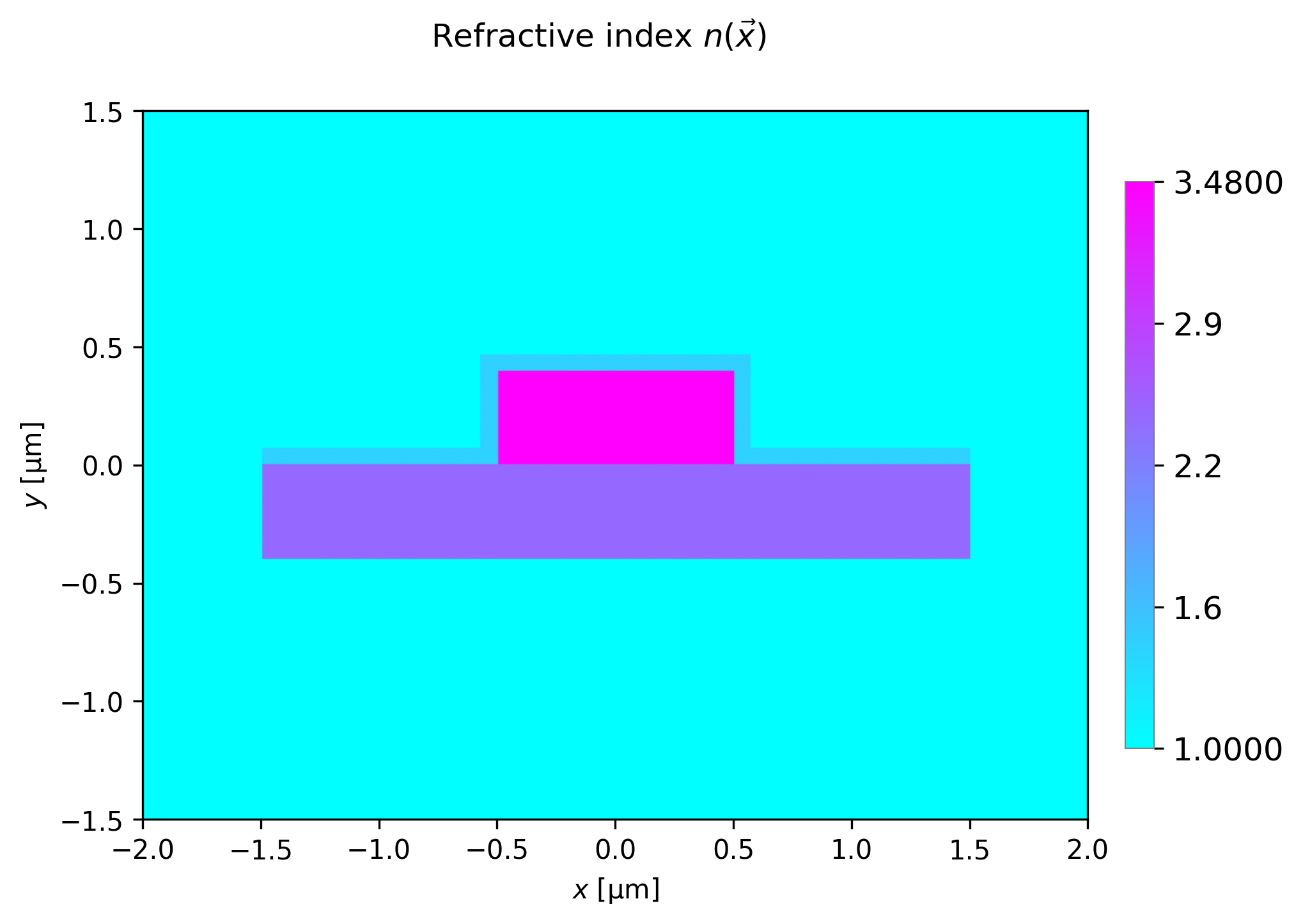
A coated rib waveguide using shape rib_coated (template rib_coated).

A rib waveguide on two substrates using shape rib_double_coated (template rib_double_coated).

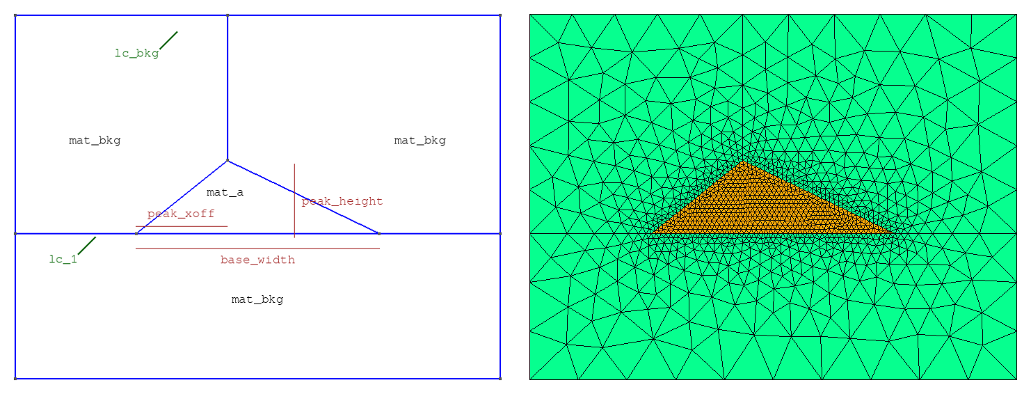
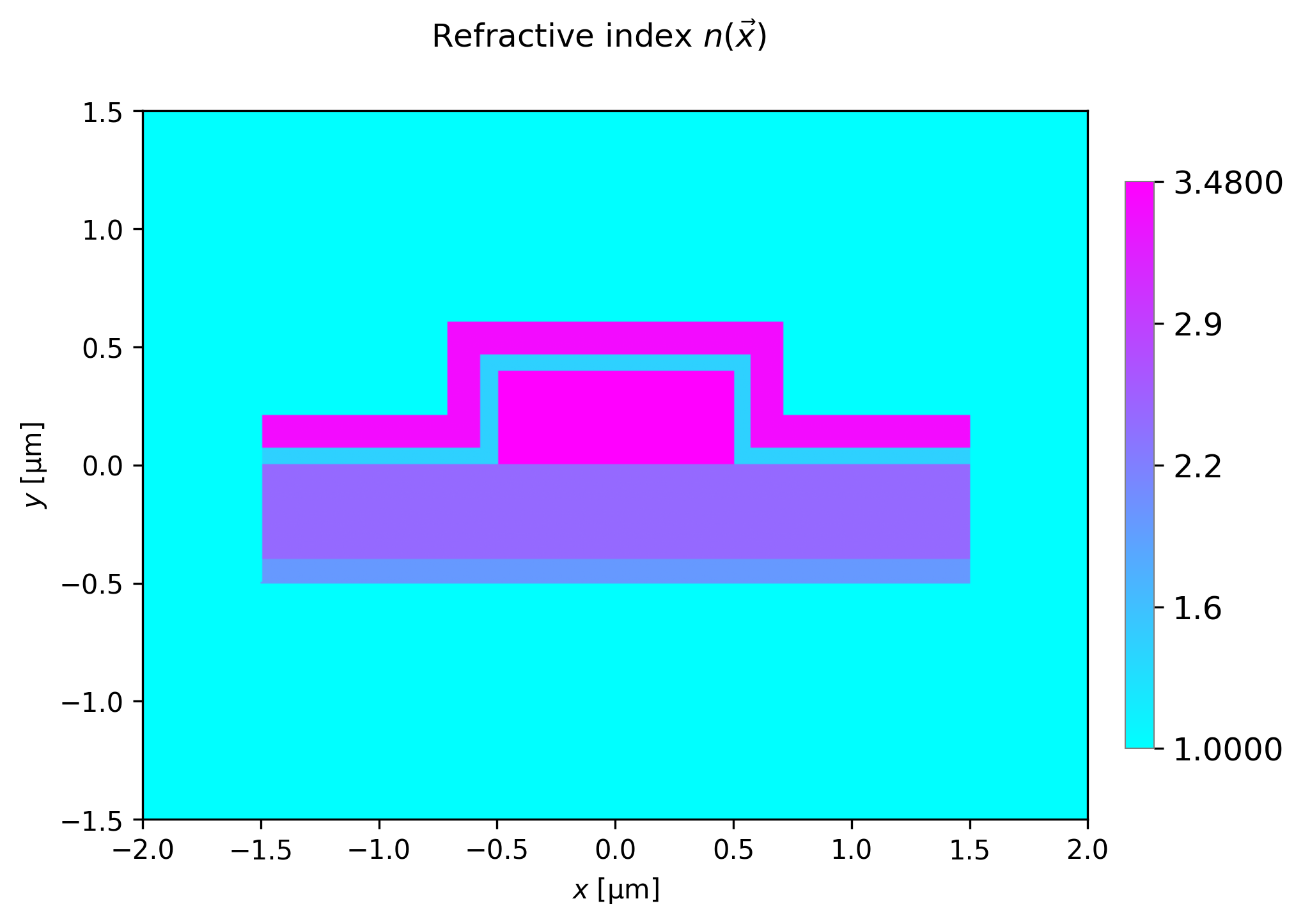
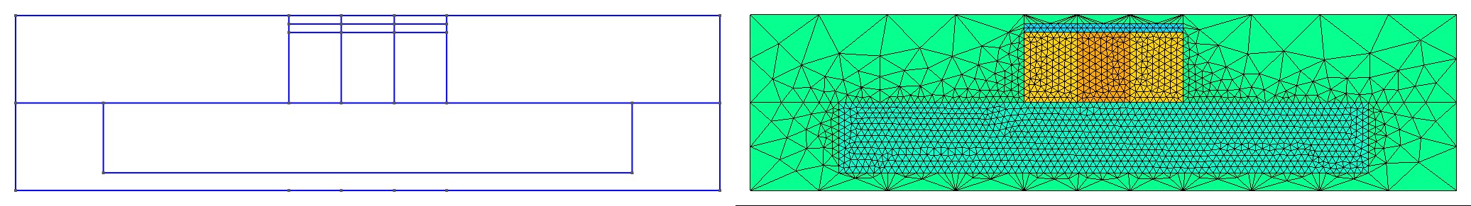
6.2.4. Engineered rib waveguides

These are examples of more complex rib geometries. These are good examples to study in order to make new designs using the user-specified waveguide and mesh mechanism.

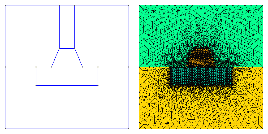
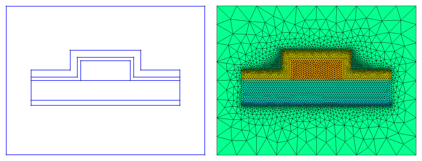
A trapezoidal rib structure using shape trapezoidal_rib.

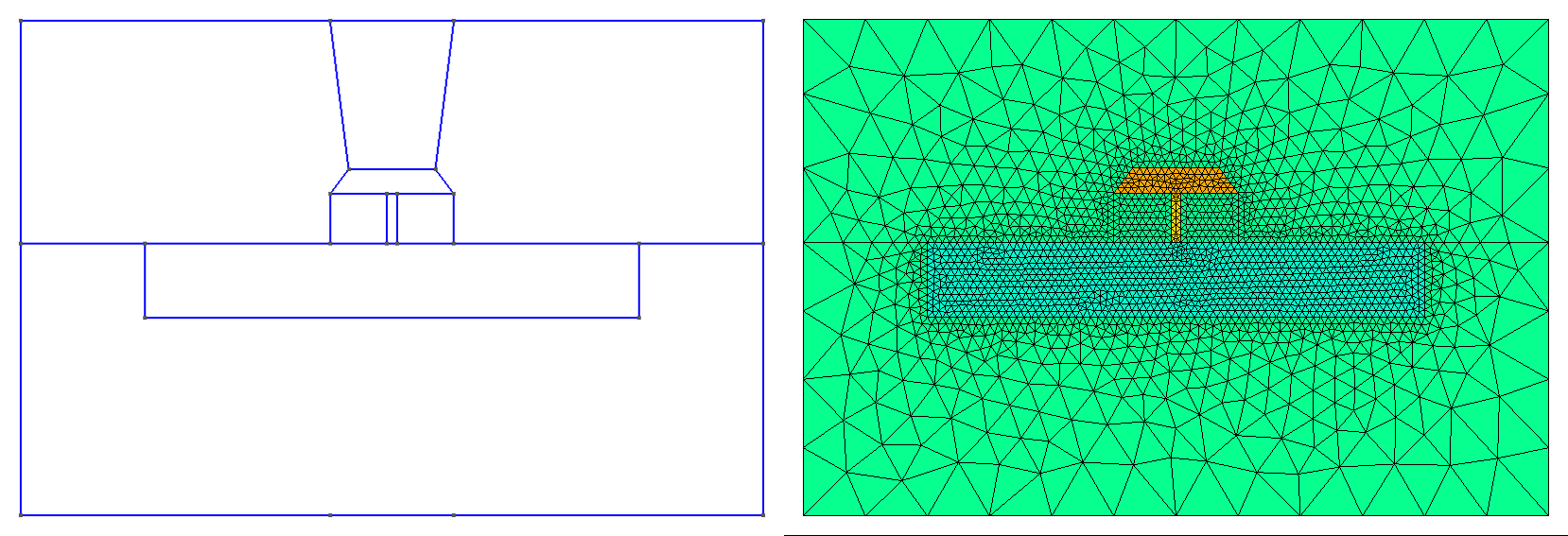
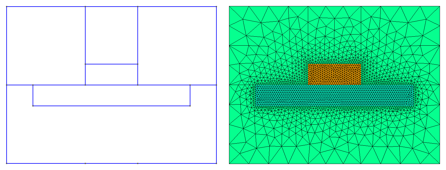
A supported pedestal structure using shape pedestal.

6.2.5. Slot waveguides

These slot waveguides can be used to enhance the horizontal component of the electric field in the low index region by the ‘slot’ effect.

A slot waveguide using shape slot (material_a is low index) (template slot).

A coated slot waveguide using shape slot_coated (material_a is low index) (template slot_coated).

6.2.6. Layered circular waveguides

These waveguides consist of a set of concentric circular rings of a desired number of layers in either a square or circular outer domain. Note that inc_a_x specifies the innermost diameter. The subsequent parameters inc_b_x, inc_c_x, etc specify the annular thickness of each successive layer.

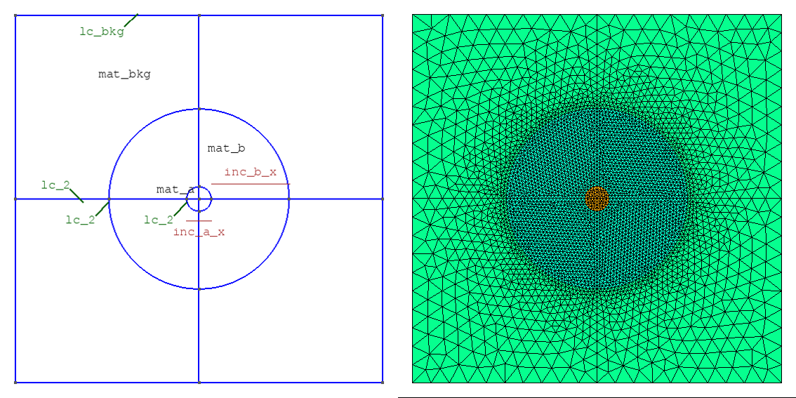
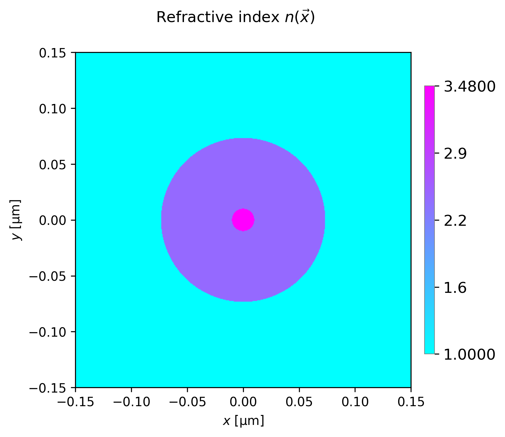
A two-layered concentric structure with background using shape onion2 (template onion2).

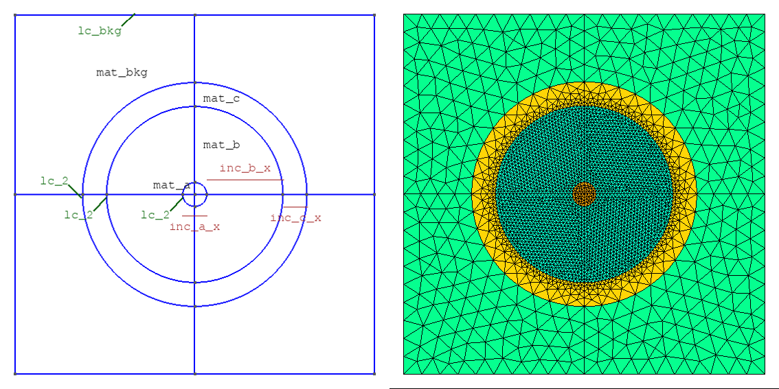
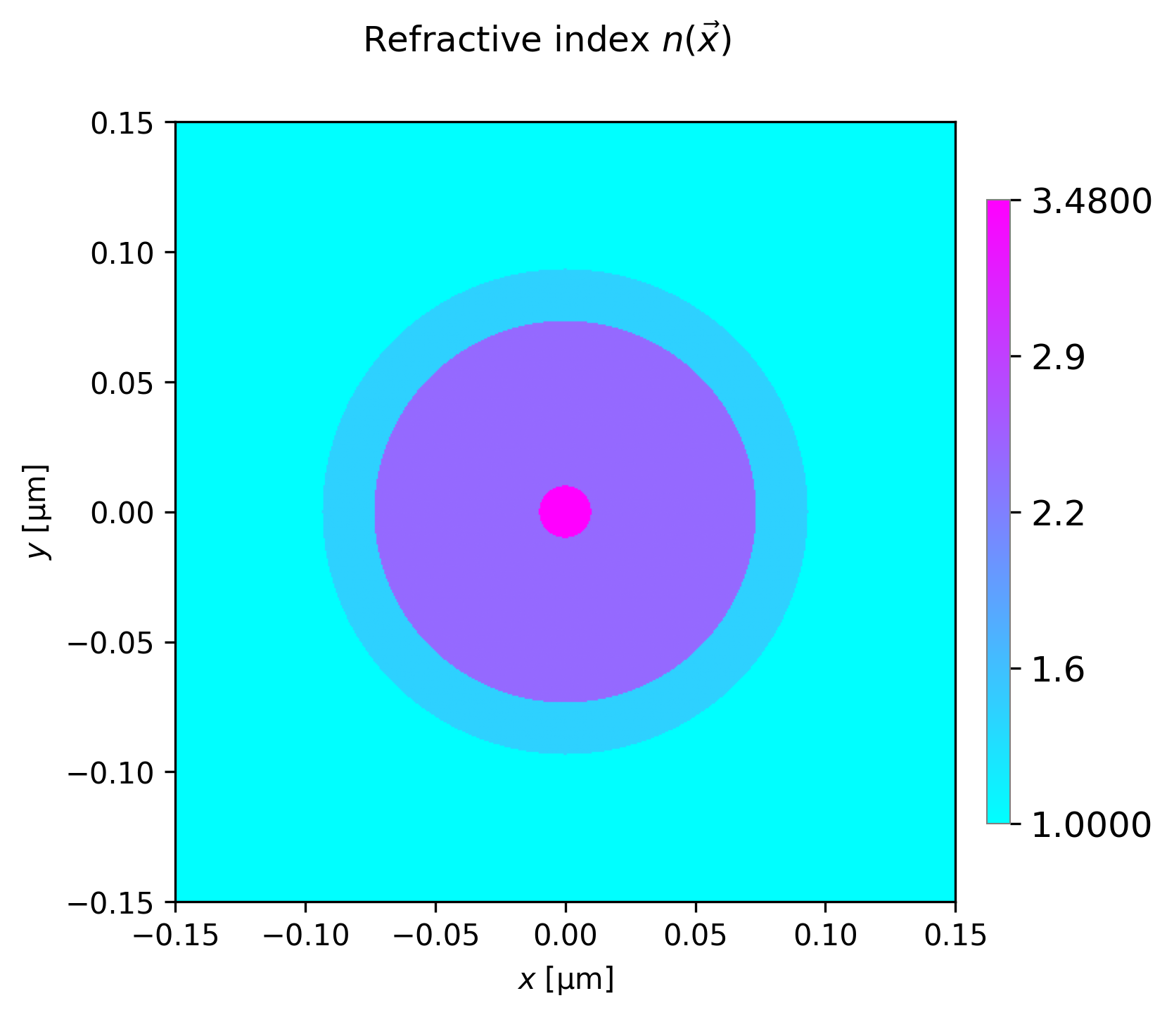
A three-layered concentric structure with background using shape onion3 (template onion3).

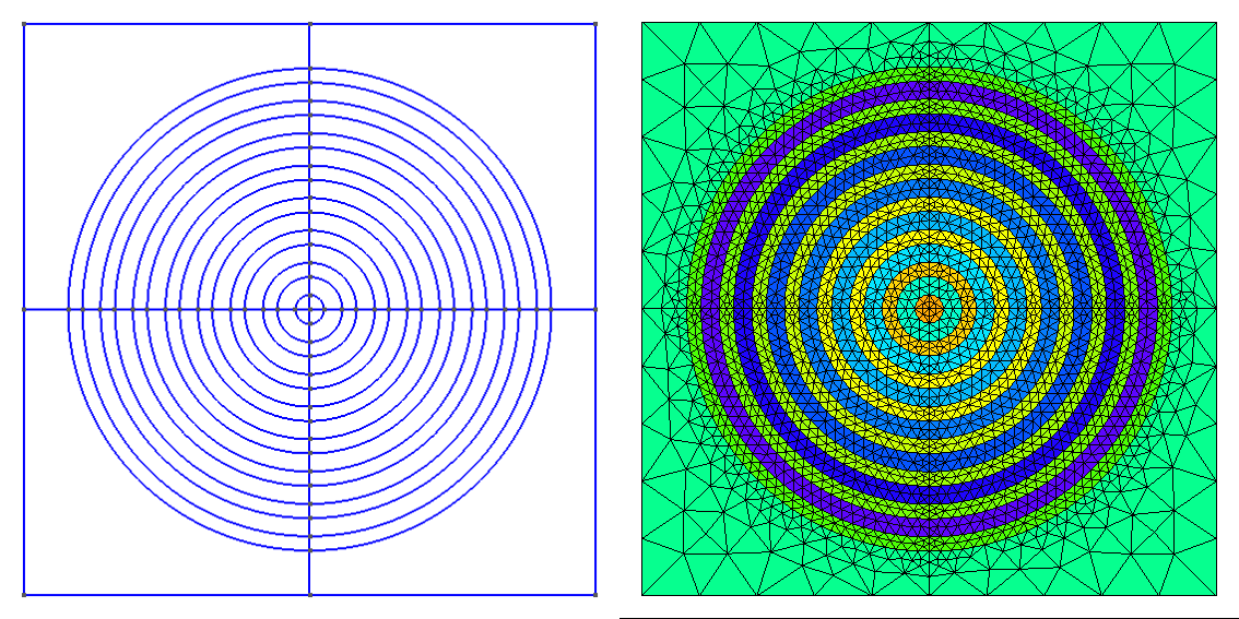
A many-layered concentric structure using shape onion (template onion).

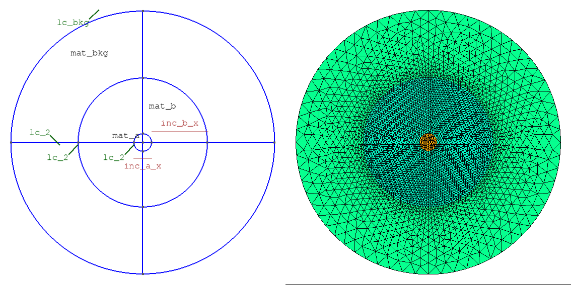
A two-layered concentric structure with a circular outer boundary using shape circ_onion2 (template circ_onion2).

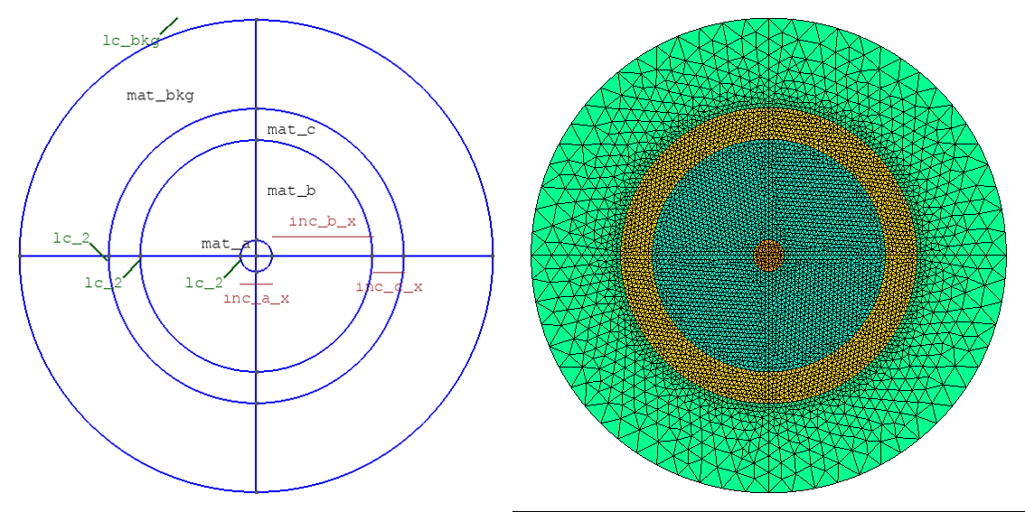
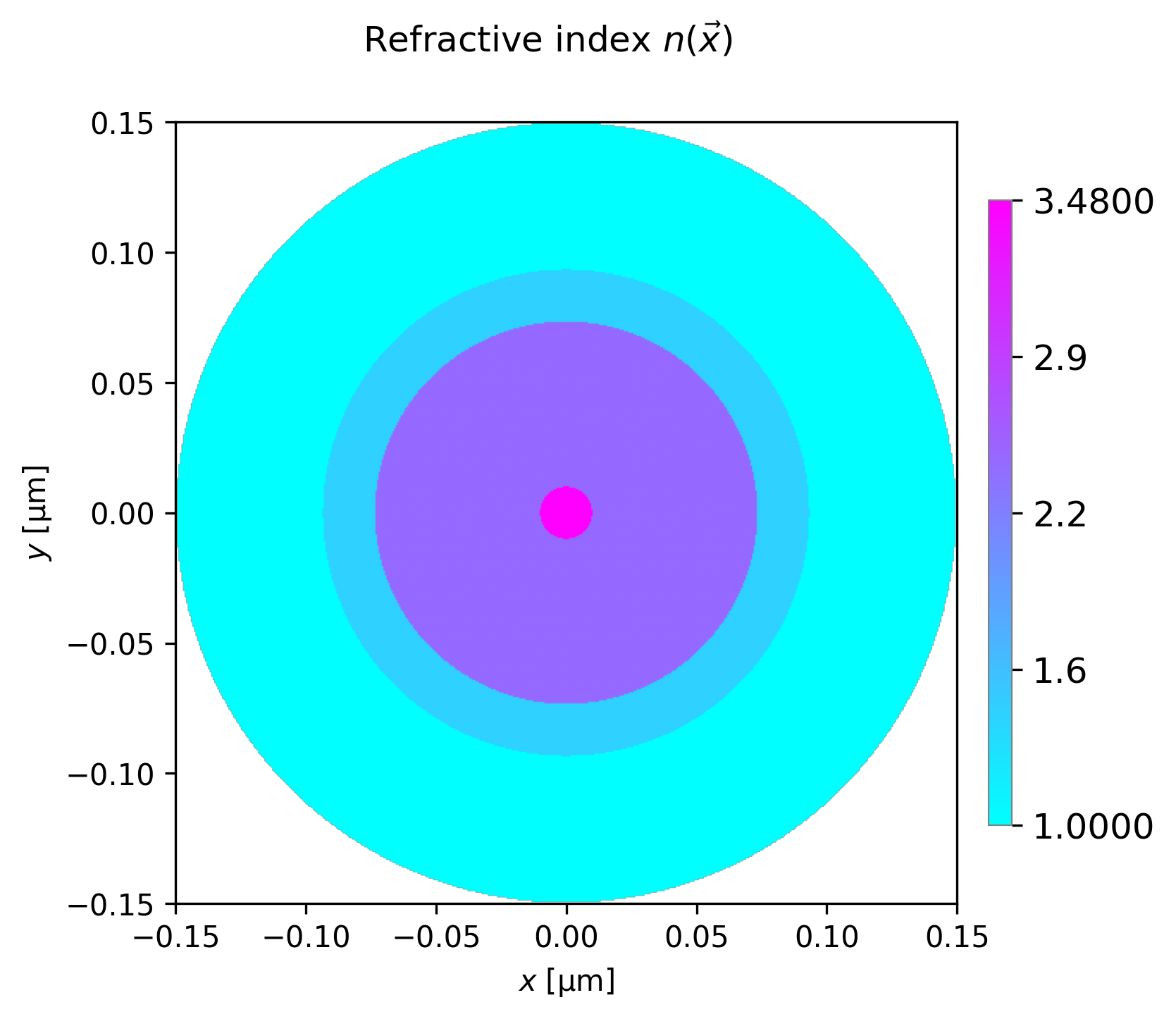
A three-layered concentric structure with a circular outer boundary using shape circ_onion3 (template circ_onion3).

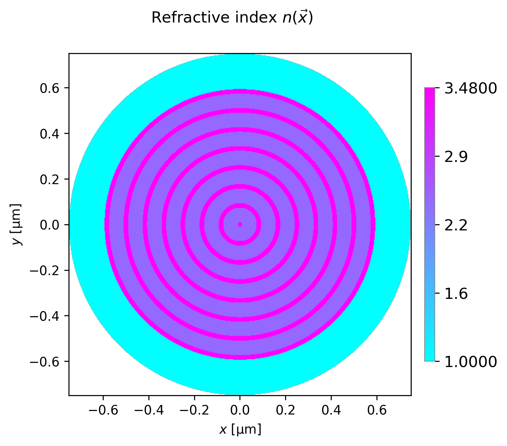
A many-layered concentric structure with a circular outer boundary using shape circ_onion (template circ_onion).

6.3. User-defined waveguide geometries

Users may incorporate their own waveguide designs fully into NumBAT with the following steps. The triangular built-in structure is a helpful model to follow.

• Create a new gmsh template .geo file to be placed in <NumBAT>/backend/msh that specifies the general structure. Start by looking at the structure of triangular_msh_template.geo and some other files to get an idea of the general structure. We’ll suppose the file is called mywaveguide_msh_template.geo and the template name is thus mywaveguide.

  When designing your template, please ensure the following:

  • That you use appropriate-sized parameters for all significant dimensions. This makes it easier to determine if the template structure has the right general shape, even though the precise dimensions will usually be changed through NumBAT calls.

  • That all Line elements are unique. In other words do not create two Line structure joining the same two points. This will produce designs that look correct, but lead to poorly formed meshes that will fail when NumBAT runs.

  • That all Line Loop elements defining a particular region are defined with the same handedness. The natural choice is to go around the loop anti-clockwise. Remember to include a minus sign for any line element that is traversed in the backwards sense.

  • That all regions that define a single physical structure with a common material are grouped together as a single Surface and then Physical Surface.

  • That the outer boundary is grouped as a Line Loop and then a Physical Line.

  • That the origin of coordinates is placed in a sensible position, such as a symmetry point close to where you expect the fundamental mode fields to be concentrated. This doesn’t actually affect NumBAT calculations but will produce more natural axis scales in output plots.

  You can see all examples of these principles followed in the mesh structures supplied with NumBAT.

• If this is your first, user-defined geometry, copy the file ‘’user_waveguides.json_template`` in <NumBAT>/backend/msh/ to user_waveguides.json in the same directory. This will ensure that subsequent git pull commands will not overwrite your work.

• Open the file user_waveguides.json and add a new dictionary element for your new waveguide, copying the general format of the pre-defined example entries.

• Fill in values for the wg_impl (the name of the python file implementing your waveguide geometry), wg_class (the name of the python class corresponding to your waveguide) and inc_shape (the waveguide template name) fields.

  • The value of inc_shape will normally be the your chosen template name, in this case mywaveguide. The other parameters can be chosen as you wish. It is natural to choose a class name which matches your template name, so perhaps MyWaveguide. However, depending on the number of geometries you create, it may be convenient to store all your classes in one python file so the filename for wg_impl may be the same for all your entries.

  • The active field allows a waveguide to be disabled if it is not yet fully working and you wish to use other NumBAT models in the meantime. You must set active to True of 1 in order to test your waveguide model.

  • Then save and close this file.

• Open or create the python file you just specified in the wg_impl field. This file must be placed in the <NumBAT>/backend/msh directory.

  • The python file must include the import line from usermesh import UserGeometryBase.

  • Create your waveguide class MyWaveguide by subclassing the UserGeometryBase class and adding init_geometry and apply_parameters methods using the Triangular class in builtin_meshes.py as a model. Both methods must take only self as arguments.

  • The init_geometry method specifies a few values including the name of the template .geo file, the number of distinct waveguide components and a short description.

  • The apply_parameters method is the mechanism for associating standard NumBAT symbols like inc_a_x, slab_a_y, etc with actual dimensions in your .geo file. This is done by string substitution of unique expressions in your .geo file using float values evaluated from the NumBAT parameters. Again, look at the examples in the Triangular class to see how this works.

  • Optionally, you may also add a draw_mpl_frame method. This provides a mechanism to draw waveguide outlines onto mode profile images and will be called automatically any time an electromagnetic or elastic mode profile is generated. The built-in waveguides Circular, Rectangular and TwoIncl provide good models for this method.

Designing and implementing a few waveguide structure should not be a daunting task but some steps can be confusing the first time round. If you hit any hiccups or have suggestions for trouble-shooting, please let us know.

6.4. Mesh parameters

The parameters lc_bkg, lc_refine_1, lc_refine_2 labelled in the above figures control the fineness of the FEM mesh and are set when constructing the waveguide, as discussed in the next chapter. The first parameter lc_bkg sets the reference background mesh size, typically as a fraction of the length of the outer boundary edge. A larger lc_bkg yields a coarser mesh. Reasonable starting values are lc_bkg=0.1 (10 mesh points on the outer boundary) to lc_bkg=0.05 (20 mesh points on the outer boundary).

As well as setting the overall mesh scale with lc_bkg, one can also refine the mesh near interfaces and near select points in the domain, as may be observed in the figures in the previous section. This helps to increase the mesh resolution in regions where there the electromagnetic and acoustic fields are likely to be strong and/or rapidly varying. This is achieved using the lc_refine_n parameters as follows. At the interface between materials, the mesh is refined to have characteristic length lc_bkg/lc_refine_1, therefore a larger lc_refine_1 gives a finer mesh by a factor of lc_refine_1 at these interfaces. The meshing program Gmsh automatically adjusts the mesh size to smoothly transition from a point that has one mesh parameter to points that have other meshing parameters. The mesh is typically also refined in the vicinity of important regions, such as in the center of a waveguide, which is done with lc_refine_2, which analogously to lc_refine_1, refines the mesh size at these points as lc_bkg/lc_refine_2.

For more complicated structures, there are additional lc_refine_<n> parameters. To see their exact function, look for these expressions in the particular .geo file.

Choosing appropriate values of lc_bkg, lc_refine_1, lc_refine_2 is crucial for NumBAT to give accurate results. The appropriate values depend strongly on the type of structure being studied, and so we strongly recommended carrying out a convergence test before delving into new structures (see Tutorial 5 for an example) starting from similar parameters as used in the tutorial simulations.

As will as giving low accuracy, a structure with too coarse a mesh is often the cause of the eigensolver failing to converge in which case NumBAT will terminate with an error. If you encounter such an error, try the calculation again with a slightly smaller value for lc_bkg, or slightly higher values for the lc_refine_n parameters.

On the other hand, it is wise to begin with relatively coarse meshes. It will be apparent that the number of elements scales roughly quadratically with the lc_refine parameters and so the run-time increases rapidly as the mesh becomes finer. For each problem, some initial experimentation to identify a mesh resolution that gives reasonable convergence in acceptable simulation is usually worthwhile.

6.5. Viewing the mesh

When NumBAT constructs a waveguide, the template geo file is converted to a concrete instantiation with the lc_refine and geometric parameters adjusted to the requested values. This file is then converted into a gmsh .msh file. When exploring new structures and their convergence behaviour, it is a very good idea to view the generated mesh frequently.

You can examine the resolution of your mesh by calling the plot_mesh(<prefix>) or check_mesh() methods on a waveguide Structure object. The first of these functions saves a pair of images of the mesh to a <prefix>-mesh-annotated.png file in the local directory which can be viewed with your preferred image viewer; the second opens the mesh in a gmsh window (see Tutorial 1 above).

In addition, the .msh file generated by NumBAT in any calculation is stored in <NumBAT>/backend/fortran/msh/build and can be viewed by running the command

gmsh <msh_filename>.msh

In some error situations, NumBAT will explicitly suggest viewing the mesh and will print out the required command to do so.